Introduction

Quantum computing hardware is becoming increasingly available and accessible, opening up opportunities for early adopters to gain practical expertise in developing and deploying quantum computations. While it will be some time before the technology can offer an advantage over classical computing for real-world applications, users today can give themselves a head-start by probing the workings and performance of multiple aspects and features of the quantum computing workflow.

For example, for those of a beginner level, simply running computations on a real quantum device can help accelerate their learning process. More expert users - e.g. researchers in academia or industry - may be interested in benchmarking particular quantum algorithms for different types of problems, or comparing different hardware devices. On yet another level, developers may wish to explore and test methods of effectively deploying and managing a workflow where classical and quantum cloud resources must operate together as seamlessly as possible.

For the foreseeable future, budget will be a significant factor in any project involving quantum computing access. Most obviously, the cost of quantum computing is currently much higher than the cost of classical computing. In benchmarking studies, for instance, this imposes limitations on the number of problems or computational runs we can execute, which in turn affects the generality of the conclusions we can draw on the performance. Moreover, with larger devices now coming online, we will be tackling problems at a correspondingly greater scale. The balance of quantum computing workflows will begin to shift away from simulators, with development and prototyping increasingly performed directly on QPUs.

In this blogpost, we give a simple practical example of cost-related trade-offs that can enter a quantum computing project. We devise a simple quantum optimisation experiment, and set a budget of around $2000 to solve the problem. Using Amazon Braket, we run our experiment on the devices provided by IonQ and Rigetti. Note that for around this same budget, one could operate a dedicated, multi-core virtual machine for a whole month on the AWS classical cloud. For example, an on-demand c6g.16xlarge EC2 instance, with 64 vCPUs and 128GiB of memory, costs approximately $1600 per month .

Bin packing

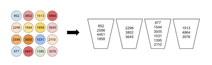
We focus on the well-known and very common problem of bin packing. We have a set of N objects, each with a given weight, and a set of M bins into which the objects must be placed. The goal is to minimise the number of bins used to store the objects; the catch is that the bins have a maximum weight capacity C, meaning that the sum of the weights assigned to each bin cannot exceed C.

To fix a specific instance of bin packing, we choose a problem comprising 8 bins and 16 objects. We set the bin capacity C = 10,000, and the object weights - drawn randomly from the range 1 to 5,000 - are shown in Figure 1. It is easy to deduce a lower bound on the number of bins needed to store the objects: simply take the sum of the object weights, divide by the bin capacity, and round up to the nearest integer. In our case, this gives a minimum bin count of 4, however this does not guarantee that a valid solution using only 4 bins exists.

A number of very simple classical heuristics exist for bin packing, which are designed to return good (but not optimal) solutions very quickly. We ran next fit, first fit, best fit, worst fit, first fit decreasing, and worst fit decreasing, with the best solution found using 5 bins. A more sophisticated classical global optimisation algorithm is simulated annealing; when given a sufficient total number of iterations (i.e. a sufficient runtime), simulated annealing does indeed find a feasible solution to our problem instance making use of only 4 bins.

Algorithm

The go-to approach for combinatorial optimisation on near-term quantum computers is undoubtedly the quantum approximate optimisation algorithm (QAOA). However, if we wish to tackle our bin packing instance on the QPUs currently available, we will need an alternative algorithm. The reason is simple: with standard QAOA, we require one qubit for every corresponding binary decision variable in our problem, however the most straightforward binary encoding for bin packing requires NM variables. Therefore, to solve our problem using QAOA, we would require at least 16 x 8 = 128 qubits, and potentially even more in order to deal with the bin capacity constraint. However, at the time of writing, the largest quantum computer available through Amazon Braket (and indeed through any public cloud provider), Rigetti’s Aspen-M1 device, contains only 80 qubits.

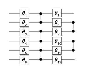
Instead, we opt for a variational quantum algorithm that trades space complexity for time complexity. Specifically, we use the basis vectors of a quantum state to represent the decision variables in our problem. The circuit requires just six qubits, and is illustrated in Figure 2. It comprises a set of single-qubit Y-rotations with variable parameters to be tuned, and a fixed set of two-qubit entangling gates (see Reference 1 ).

Execution

We ran our bin packing problem on two quantum computers accessed through AWS Braket - IonQ’s 11-qubit trapped ion device, and Rigetti’s Aspen-9 32-qubit superconducting chip (since replaced by the larger M1 device). We performed all parameter training on the QPUs, using a gradient-based classical optimiser, SPSA , to search for the optimal circuit parameters. This is an economical approach, since it requires only two function evaluations at each optimiser iteration, independent of the number of variational parameters. In other words, we need only execute two quantum circuits at each optimiser iteration, which keeps both the per-task and per-shot costs to a minimum.

We cap the number of optimiser iterations at 100, meaning we must execute a total of 200 circuits (tasks) each time we run the computation. For each circuit, we take 1000 shots to obtain the probability distribution over the possible outcomes. At current prices, this means we spend $2060 to run the problem on IonQ’s 11-qubit device, and $130 for Rigetti’s 32-qubit Aspen-9 device.

Since there is an approximately 16-fold difference in cost, in principle we can then run the same problem 16 times on Rigetti, and still maintain cost parity. However, the Rigetti device in fact has 32 qubits, so we can actually execute several instances of our 6-qubit problem in parallel. In order to maintain some degree of physical separation between the different sets of 6 qubits on the chip (and thus ideally minimise the impact of cross-talk errors), we choose to run 4 concurrent problem instances, making use of 24 qubits in total. Therefore, we are in fact able to run our problem 64 times on Rigetti at the same cost as a single run on IonQ.

A natural question is then, how might we use the additional runs available with Rigetti? We will explore two options in this blogpost. The first is simply to run the computation with 64 different sets of initial circuit parameters, or ‘seeds’, which we generate randomly. The second is to explore different hyperparameter settings of the SPSA optimiser. Specifically, we consider 4 different values of the angular update Δθ at the first optimiser iteration, following the method discussed in Reference 2 . We are then able to run 16 seeds for each hyperparameter set.

Before proceeding, we give one additional example of a different way to exploit the lower pricing of the Rigetti device, which we do not consider in our experiments for this blogpost. Specifically, the number of shots taken to obtain the probability distribution is another hyperparameter of our algorithm. By taking more shots, we could reduce the error in our estimate of the cost function value for a given set of circuit parameters. In turn, this may be beneficial for the optimisation process itself.

Results

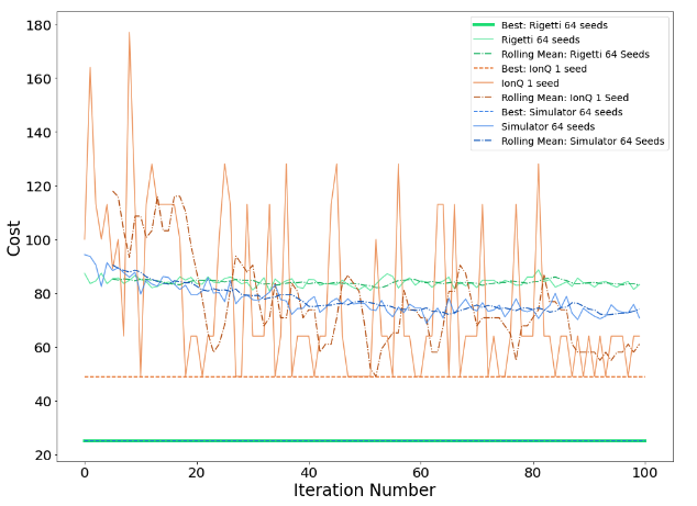
Figure 3 shows our various results using a fixed value of the initial angular update, Δθ = 0.005. In our convention, a cost value of 64 or lower is a feasible solution to the problem, i.e. all objects are assigned to a bin, and no bin exceeds its maximum capacity. We first simulated the outcome using the noiseless statevector simulator included in the Braket SDK. The results of this show that the mean cost over the 64 seeds has a clear downward trend, and after 100 iterations is approaching the feasible region. This indicates that our toy algorithm is perhaps best seen as a means of finding constraint-satisfying solutions, rather than finding the global minimum.

Turning to the results from Rigetti’s device, we see that the average cost of the same 64 seeds remains effectively constant across the 100 iterations. Nevertheless, the best individual result found has a cost that corresponds to using 5 bins, which coincides with the result of the best classical heuristic method.

Selecting one of the 64 seeds to run on IonQ, we see an overall downward trend in the cost function value, with the rolling mean value (computed over the previous 5 iterations) entering the feasible region after around 90 iterations. On the other hand, the best solutions found use a total of 7 bins. (NB: for this same single instance run on Rigetti, we saw no downward trend in the cost function value).

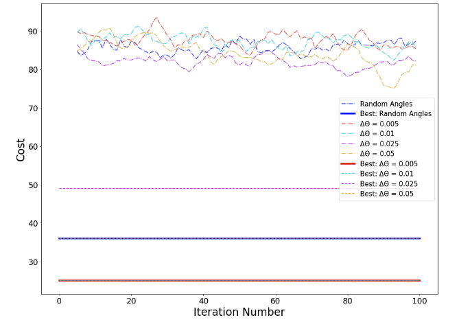
Focusing specifically on the Rigetti device, we investigate hyperparameter tuning by comparing four values of Δθ, in each case averaging over 16 different random seeds for the initial circuit parameters. Figure 4 shows the rolling mean of the cost function value over the previous 5 iterations. With Δθ = 0.025 we observe an improvement of around 4% in the cost function value, compared with the original choice of Δθ = 0.005. Meanwhile, the case Δθ = 0.05 appears to show a slow downward trend in the cost, indicating that some degree of optimisation may be taking place.

For comparison, we also considered a simple random sampling strategy, where we initialise each circuit with a random set of angles, and immediately compute the cost function value according to the digitisation procedure. We see that the results of this random sampling are generally similar to those obtained using SPSA on the Rigetti device.

Summary and outlook

We have explored different options for solving a small toy optimisation problem within a fixed budget through Amazon Braket, using devices provided by IonQ and Rigetti. The lower pricing of the Rigetti superconducting qubit device allows a wider exploration of algorithm hyperparameters. Here, we considered those related to the classical optimisation component, and in doing so we found a small improvement in the performance. IonQ’s trapped ion device is significantly more expensive to access, limiting the scope for algorithmic fine tuning. Nevertheless, overall there is a much clearer trend in optimisation of the objective function.

As larger quantum computers become available, simulating the outcomes of our algorithms will become impractical or impossible. Key tasks such as benchmarking, or algorithmic prototyping - including hyperparameter tuning, which is a common component of optimisation and machine learning workflows - will increasingly need to be performed directly on QPUs themselves. Many quantum computing projects will be constrained significantly by budget, and as we have shown by example in this blogpost, this means that users will need to carefully consider the trade-off between the scope and the cost of what they wish to achieve.

References

1. C. Bravo-Prieto et al, Quantum 4, 272 (2020) .

2. A. Kandala et al, arXiv:1704.05018v2 , (supplementary material, section VI).